Linear Regression

Mục tiêu bài học

Sau bài học này, học viên sẽ:

• Hiểu bản chất cua Linear Regression
• Nắm vững công thức OLS (Ordinary Least Squares)
• Tính toán thủ công Linear Regression
• Implement với Scikit-learn

1. Giới thiệu Linear Regression

1.1 Ý tưởng

Linear Regression tìm đường thẳng tốt nhất để mô tả mối quan hệ giữa biến độc lập (X) va biến phụ thuộc (y).

Công thức:

$\hat{y} = \beta_0 + \beta_1 x$

Trong do:

• $\hat{y}$: Gia tri dự đoán
• $\beta_0$: Intercept (hệ số chặn)
• $\beta_1$: Slope (hệ số góc)
• $x$: Bien doc lap

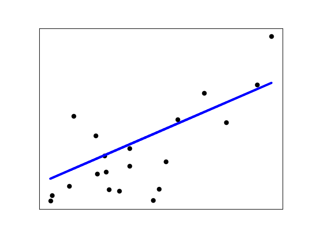
Hinh: Linear Regression fit đường thẳng qua các điểm du lieu

1.2 Multiple Linear Regression

Với nhiều biến:

$\hat{y} = \beta_0 + \beta_1 x_1 + \beta_2 x_2 + ... + \beta_n x_n$

Hoac dạng ma trận:

$\hat{y} = X\beta$

2. Ordinary Least Squares (OLS)

2.1 Mục tiêu

Tim $\beta$ sao cho tổng bình phương sai số la nhỏ nhất:

$J(\beta) = \sum_{i=1}^{m}(y_i - \hat{y}_i)^2 = \sum_{i=1}^{m}(y_i - \beta_0 - \beta_1 x_i)^2$

2.2 Công thức OLS

Slope:

$\beta_1 = \frac{\sum_{i=1}^{m}(x_i - \bar{x})(y_i - \bar{y})}{\sum_{i=1}^{m}(x_i - \bar{x})^2} = \frac{Cov(X, Y)}{Var(X)}$

Intercept:

$\beta_0 = \bar{y} - \beta_1 \bar{x}$

2.3 Dang ma tran

$\beta = (X^T X)^{-1} X^T y$

3. Ví dụ tính toán thủ công

3.1 Dữ liệu

3.2 Bước 1: Tính Mean

$\bar{x} = \frac{50+60+70+80+100}{5} = \frac{360}{5} = 72$

$\bar{y} = \frac{500+600+650+700+850}{5} = \frac{3300}{5} = 660$

3.3 Bước 2: Tính các thành phần

3.4 Bước 3: Tính hệ số

Slope:

$\beta_1 = \frac{9900}{1480} = 6.69$

Intercept:

$\beta_0 = 660 - 6.69 \tìmes 72 = 660 - 481.68 = 178.32$

3.5 Bước 4: Phương trình hồi quy

$\hat{y} = 178.32 + 6.69x$

Diễn giải: Mỗi mét vuông tăng thêm, giá tăng 6.69 triệu VND.

3.6 Bước 5: Du doan

Với nhà 90m2:

$\hat{y} = 178.32 + 6.69 \tìmes 90 = 178.32 + 602.1 = 780.42 \text{ triệu VND}$

4. Đánh giá Model

4.1 Mean Squared Error (MSE)

$MSE = \frac{1}{m}\sum_{i=1}^{m}(y_i - \hat{y}_i)^2$

4.2 Root Mean Squared Error (RMSE)

$RMSE = \sqrt{MSE}$

4.3 R-squared (R2)

$R^2 = 1 - \frac{SS_{res}}{SS_{tot}} = 1 - \frac{\sum(y_i - \hat{y}_i)^2}{\sum(y_i - \bar{y})^2}$

5. Thực hành với Scikit-learn

5.1 Code hoàn chỉnh

1import numpy as np
2import matplotlib.pyplot as plt
3from sklearn.linear_model import LinearRegression
4from sklearn.model_selection import train_test_split
5from sklearn.metrics import mean_squared_error, r2_score
6
7# Dữ liệu
8X = np.array([50, 60, 70, 80, 100]).reshape(-1, 1)
9y = np.array([500, 600, 650, 700, 850])
10
11# Train model
12model = LinearRegression()
13model.fit(X, y)
14
15# Xem hệ số
16print(f"Intercept (beta_0): {model.intercept_:.2f}")
17print(f"Slope (beta_1): {model.coef_[0]:.2f}")
18
19# Du doan
20y_pred = model.predict(X)
21print(f"Predictions: {y_pred}")
22
23# Đánh giá
24mse = mean_squared_error(y, y_pred)
25rmse = np.sqrt(mse)
26r2 = r2_score(y, y_pred)
27
28print(f"MSE: {mse:.2f}")
29print(f"RMSE: {rmse:.2f}")
30print(f"R2: {r2:.4f}")
31
32# Visualize
33plt.figure(figsize=(10, 6))
34plt.scatter(X, y, color='blue', label='Actual')
35plt.plot(X, y_pred, color='red', label='Predicted')
36plt.xlabel('Diện tích (m2)')
37plt.ylabel('Gia (triệu VND)')
38plt.title('Linear Regression - House Price Prediction')
39plt.legend()
40plt.grid(True)
41plt.show()

5.2 Multiple Linear Regression

1from sklearn.datasets import fetch_california_housing
2from sklearn.model_selection import train_test_split
3from sklearn.linear_model import LinearRegression
4from sklearn.metrics import mean_squared_error, r2_score
5from sklearn.preprocessing import StandardScaler
6
7# Load data
8housing = fetch_california_housing()
9X, y = housing.data, housing.target
10
11# Split
12X_train, X_test, y_train, y_test = train_test_split(
13    X, y, test_size=0.2, random_state=42
14)
15
16# Scale (quan trong cho multiple regression)
17scaler = StandardScaler()
18X_train_scaled = scaler.fit_transform(X_train)
19X_test_scaled = scaler.transform(X_test)
20
21# Train
22model = LinearRegression()
23model.fit(X_train_scaled, y_train)
24
25# Predict
26y_pred = model.predict(X_test_scaled)
27
28# Evaluate
29print(f"R2 Score: {r2_score(y_test, y_pred):.4f}")
30print(f"RMSE: {np.sqrt(mean_squared_error(y_test, y_pred)):.4f}")
31
32# Feature importance
33for name, coef in zip(housing.feature_names, model.coef_):
34    print(f"{name}: {coef:.4f}")

6. Giả định của Linear Regression

6.1 Cac gia dinh

6.2 Kiểm tra Residuals

1import matplotlib.pyplot as plt
2import scipy.stats as stats
3
4# Tính residuals
5residuals = y_test - y_pred
6
7# Residual plot
8plt.figure(figsize=(12, 4))
9
10plt.subplot(1, 2, 1)
11plt.scatter(y_pred, residuals)
12plt.axhline(y=0, color='r', linestyle='--')
13plt.xlabel('Predicted')
14plt.ylabel('Residuals')
15plt.title('Residual Plot')
16
17# Q-Q plot
18plt.subplot(1, 2, 2)
19stats.probplot(residuals, dist="norm", plot=plt)
20plt.title('Q-Q Plot')
21
22plt.tight_layout()
23plt.show()

7. Ưu và nhược điểm

Bài tập tự luyện

1. Bai tap 1: Tính thu cong Linear Regression voi data: X=[1,2,3,4,5], y=[2,4,5,4,5]
2. Bai tap 2: Load Boston Housing dataset, train Linear Regression, danh gia R2
3. Bai tap 3: Kiểm tra cac gia dinh cua Linear Regression voi residual plots

Tài liệu tham khảo

• Scikit-learn Linear Regression
• StatQuest - Linear Regression
• OLS Wikipedia