🎯 Mục tiêu bài học
Sau bài học này, học viên sẽ:
✅ Hiểu sự khác biệt giữa Supervised và Unsupervised Learning
✅ Nắm vững thuật toán K-Means Clustering
✅ Hiểu PCA (Principal Component Analysis)
✅ Biết cách phát hiện bất thường (Anomaly Detection)
Thời gian: 5-6 giờ | Độ khó: Theory
� Bảng Thuật Ngữ Quan Trọng
| Thuật ngữ | Tiếng Việt | Giải thích đơn giản |
|---|---|---|
| Unsupervised Learning | Học không giám sát | Học từ data không có label |
| Clustering | Phân cụm | Nhóm các điểm dữ liệu tương tự |
| K-Means | K-Means | Thuật toán clustering phổ biến nhất |
| Centroid | Tâm cụm | Điểm trung tâm của cluster |
| Elbow Method | Phương pháp khuỷu tay | Chọn k tối ưu dựa trên inertia |
| PCA | Phân tích thành phần chính | Giảm chiều giữ variance |
| Anomaly Detection | Phát hiện bất thường | Tìm outlier/fraud |
| Silhouette Score | Điểm Silhouette | Đo chất lượng clustering |
Checkpoint
Bạn đã đọc qua bảng thuật ngữ? Hãy ghi nhớ chúng!
�📊 Tổng quan Unsupervised Learning
1. Tổng quan Unsupervised Learning
1.1 So sánh với Supervised Learning
| Tiêu chí | Supervised | Unsupervised |
|---|---|---|
| Label | Có y | Không có y |
| Mục tiêu | Predict | Discover patterns |
| Ví dụ | Classification, Regression | Clustering, Dimensionality Reduction |
1.2 Các loại bài toán
- Clustering: Nhóm data points tương tự
- Dimensionality Reduction: Giảm số chiều
- Anomaly Detection: Phát hiện điểm bất thường
🎯 K-Means Clustering
2. K-Means Clustering
2.1 Ý tưởng chính
K-Means chia data thành K clusters sao cho:
- Các điểm trong cùng cluster gần nhau
- Các điểm khác cluster xa nhau
Objective Function (Inertia):
2.2 Thuật toán K-Means
Các bước:
| Bước | Mô tả |
|---|---|
| 1 | Khởi tạo K centroids ngẫu nhiên |
| 2 | Gán mỗi điểm vào centroid gần nhất |
| 3 | Cập nhật centroids = trung bình các điểm trong cluster |
| 4 | Lặp lại bước 2-3 cho đến khi hội tụ |
2.3 Minh họa K-Means
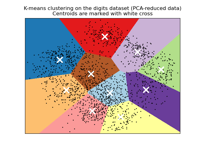
Hình: K-Means clustering trên MNIST digits dataset. Centroids được đánh dấu bằng dấu X trắng.
📝 Ví dụ tính K-Means thủ công
3. Vi du tinh K-Means thu cong
3.1 Data và khởi tạo
Data points:
| Point | X | Y |
|---|---|---|
| P1 | 1 | 1 |
| P2 | 1.5 | 2 |
| P3 | 3 | 4 |
| P4 | 5 | 7 |
| P5 | 3.5 | 5 |
| P6 | 4.5 | 5 |
K = 2, khởi tạo:
- Centroid 1 = P1 = (1, 1)
- Centroid 2 = P4 = (5, 7)
3.2 Iteration 1: Gán điểm
Tính khoang cach Euclidean:
| Point | dist to C1 | dist to C2 | Cluster |
|---|---|---|---|
| P1 | 0 | 7.21 | C1 |
| P2 | 1.12 | 6.10 | C1 |
| P3 | 3.61 | 3.61 | C1 |
| P4 | 7.21 | 0 | C2 |
| P5 | 4.72 | 2.50 | C2 |
| P6 | 5.32 | 2.06 | C2 |
3.3 Iteration 1: Cập nhật Centroid
Cluster 1: P1, P2, P3
Cluster 2: P4, P5, P6
3.4 Iteration 2: Gán lại
| Point | dist to C1 | dist to C2 | Cluster |
|---|---|---|---|
| P1 | 1.56 | 5.69 | C1 |
| P2 | 0.47 | 4.68 | C1 |
| P3 | 2.04 | 1.99 | C2 |
| P4 | 5.48 | 1.49 | C2 |
| P5 | 3.11 | 1.02 | C2 |
| P6 | 3.69 | 0.67 | C2 |
Kết quả: Point P3 chuyển từ C1 sang C2!
3.5 Cập nhật và hội tụ
Cluster 1: P1, P2
Cluster 2: P3, P4, P5, P6
Tiếp tục cho đến khi centroids khong doi.
Checkpoint
Bạn có thể tính toán thủ công một iteration của K-Means không?
📉 Elbow Method - Chọn K
4. Elbow Method - Chọn K
4.1 Ý tưởng
Chọn K tại điểm "khuỷu tay" - nơi giảm Inertia chậm lại đáng kể.
4.2 Minh hoa Elbow Method

Hinh: Elbow Method - Chọn K tại điểm uốn cong.
4.3 Ví dụ tính Inertia
| K | Inertia | Giảm |
|---|---|---|
| 1 | 100 | - |
| 2 | 50 | 50 |
| 3 | 30 | 20 |
| 4 | 25 | 5 |
| 5 | 23 | 2 |
Chọn K = 4 vi sau đó inertia giảm rất ít.
💻 Thực hành K-Means
5. Thuc hanh K-Means
5.1 Code hoàn chỉnh
1import numpy as np2import matplotlib.pyplot as plt3from sklearn.cluster import KMeans4from sklearn.preprocessing import StandardScaler5from sklearn.datasets import make_blobs67# Tạo data8X, y_true = make_blobs(n_samples=300, centers=4, random_state=42)910# Scale data11scaler = StandardScaler()12X_scaled = scaler.fit_transform(X)1314# Elbow Method15inertias = []16K_range = range(1, 11)1718for k in K_range:19 kmeans = KMeans(n_clusters=k, random_state=42, n_init=10)20 kmeans.fit(X_scaled)21 inertias.append(kmeans.inertia_)2223# Vẽ Elbow24plt.figure(figsize=(10, 4))25plt.subplot(1, 2, 1)26plt.plot(K_range, inertias, 'bo-')27plt.xlabel('K')28plt.ylabel('Inertia')29plt.title('Elbow Method')3031# K-Means voi K tối ưu32k_optìmal = 433kmeans = KMeans(n_clusters=k_optìmal, random_state=42, n_init=10)34labels = kmeans.fit_predict(X_scaled)3536# Visualize37plt.subplot(1, 2, 2)38plt.scatter(X_scaled[:, 0], X_scaled[:, 1], c=labels, cmap='viridis')39plt.scatter(kmeans.cluster_centers_[:, 0], 40 kmeans.cluster_centers_[:, 1], 41 c='red', marker='x', s=200, linewidths=3)42plt.title('K-Means Clustering')43plt.tight_layout()44plt.show()4546# Đánh giá47from sklearn.metrics import silhouette_score48sil_score = silhouette_score(X_scaled, labels)49print(f"Silhouette Score: {sil_score:.4f}")5.2 Silhouette Score
Đánh giá chat luong clustering:
Trong do:
- a(i): Khoang cach trung binh đến cac điểm cung cluster
- b(i): Khoang cach trung binh đến cluster gan nhat
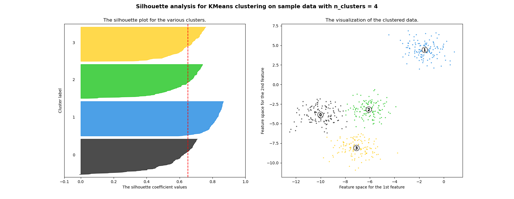
Hinh: Silhouette analysis cho K-Means clustering.
| Silhouette | Interpretation |
|---|---|
| 0.7 - 1.0 | Excellent |
| 0.5 - 0.7 | Good |
| 0.25 - 0.5 | Fair |
| less than 0.25 | Poor |
📊 PCA - Principal Component Analysis
6. PCA - Principal Component Analysis
6.1 Ý tưởng chinh
Giảm so chieu data trong khi giu lai phuong sai lon nhat.
6.2 Minh hoa PCA
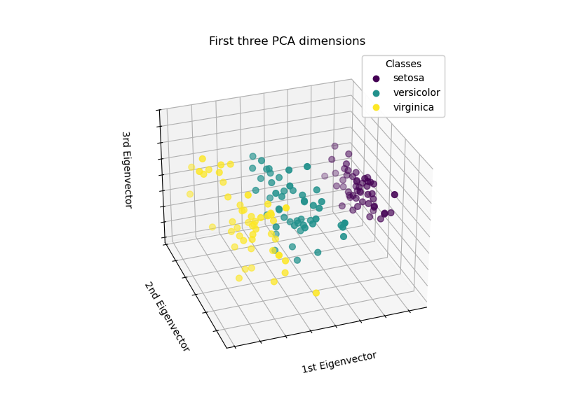
Hinh: PCA projection 3D cua Iris dataset - Tu 4 features xuong 3 principal components.
6.3 Thuật toán PCA
| Bước | Mô tả |
|---|---|
| 1 | Standardize data (mean=0, std=1) |
| 2 | Tính Covariance Matrix |
| 3 | Tính Eigenvalues va Eigenvectors |
| 4 | Chọn top-k eigenvectors |
| 5 | Transform data |
6.4 Công thức
Covariance Matrix:
Eigenvalue Equation:
Explained Variance Ratio:
📝 Ví dụ PCA thủ công
7. Vi du PCA thu cong
7.1 Data 2D
| X1 | X2 |
|---|---|
| 2.5 | 2.4 |
| 0.5 | 0.7 |
| 2.2 | 2.9 |
| 1.9 | 2.2 |
| 3.1 | 3.0 |
7.2 Step 1: Standardize
Mean X1 = 2.04, Mean X2 = 2.24
Tru mean tu moi gia tri.
7.3 Step 2: Covariance Matrix
7.4 Step 3: Eigenvalues
Explained Variance:
- PC1: 96.3%
- PC2: 3.7%
PC1 giu lai 96.3% thong tin!
💻 Thực hành PCA
8. Thuc hanh PCA
8.1 Code hoàn chỉnh
1from sklearn.decomposition import PCA2from sklearn.preprocessing import StandardScaler3import numpy as np4import matplotlib.pyplot as plt5from sklearn.datasets import load_iris67# Load data8iris = load_iris()9X = iris.data10y = iris.target1112# Standardize13scaler = StandardScaler()14X_scaled = scaler.fit_transform(X)1516# PCA17pca = PCA(n_components=2)18X_pca = pca.fit_transform(X_scaled)1920# Explained Variance21print("Explained Variance Ratio:", pca.explained_variance_ratio_)22print("Total:", sum(pca.explained_variance_ratio_))2324# Cumulative Variance25pca_full = PCA()26pca_full.fit(X_scaled)27cum_var = np.cumsum(pca_full.explained_variance_ratio_)2829plt.figure(figsize=(12, 4))3031# Plot 1: Cumulative Variance32plt.subplot(1, 2, 1)33plt.plot(range(1, len(cum_var)+1), cum_var, 'bo-')34plt.axhline(y=0.95, color='r', linestyle='--', label='95%')35plt.xlabel('Number of Components')36plt.ylabel('Cumulative Variance')37plt.title('PCA - Explained Variance')38plt.legend()3940# Plot 2: 2D Visualization41plt.subplot(1, 2, 2)42scatter = plt.scatter(X_pca[:, 0], X_pca[:, 1], c=y, cmap='viridis')43plt.xlabel('PC1')44plt.ylabel('PC2')45plt.title('PCA - 2D Projection')46plt.colorbar(scatter)47plt.tight_layout()48plt.show()8.2 Minh hoa PCA vs LDA
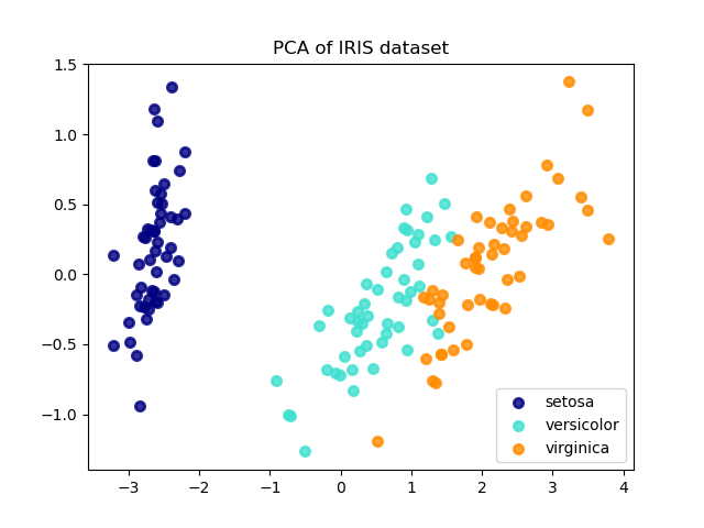
Hinh: So sanh PCA va LDA projection tren Iris dataset.
8.3 Chọn so components
1# Chọn components giu 95% variance2pca_95 = PCA(n_components=0.95)3X_reduced = pca_95.fit_transform(X_scaled)4print(f"Components needed for 95%: {pca_95.n_components_}")Checkpoint
Bạn có thể giải thích Explained Variance Ratio nghĩa là gì không?
🚨 Anomaly Detection
9. Anomaly Detection
9.1 Isolation Forest
Ý tưởng: Diem bat thuong de bi "co lap" hon điểm binh thuong.
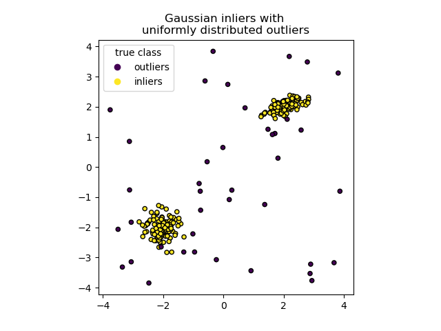
Hinh: Isolation Forest anomaly detection.
1from sklearn.ensemble import IsolationForest23# Fit model4iso_forest = IsolationForest(contamination=0.1, random_state=42)5predictions = iso_forest.fit_predict(X)67# -1: anomaly, 1: normal8anomalies = X[predictions == -1]9normal = X[predictions == 1]1011print(f"Anomalies found: {len(anomalies)}")9.2 Local Outlier Factor (LOF)
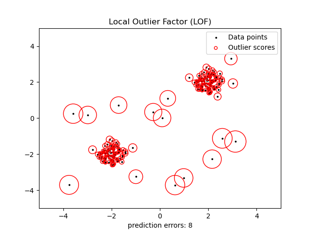
Hinh: Local Outlier Factor outlier detection.
1from sklearn.neighbors import LocalOutlierFactor23lof = LocalOutlierFactor(n_neighbors=20, contamination=0.1)4predictions = lof.fit_predict(X)56# Visualize7plt.scatter(X[:, 0], X[:, 1], c=predictions, cmap='coolwarm')8plt.title('LOF Anomaly Detection')9plt.show()⚖️ Ưu và nhược điểm
10. Ưu và nhược điểm
10.1 K-Means
| Uu điểm | Nhuoc điểm |
|---|---|
| Don gian, nhanh | Phai chon K truoc |
| Scalable | Sensitive voi outliers |
| Easy to interpret | Chi tìm spherical clusters |
10.2 PCA
| Uu điểm | Nhuoc điểm |
|---|---|
| Giảm chieu hiệu quả | Linear only |
| Loai bo noise | Kho interpret components |
| Giảm overfitting | Mat mot phan thong tin |
10.3 So sanh cac phuong phap Clustering
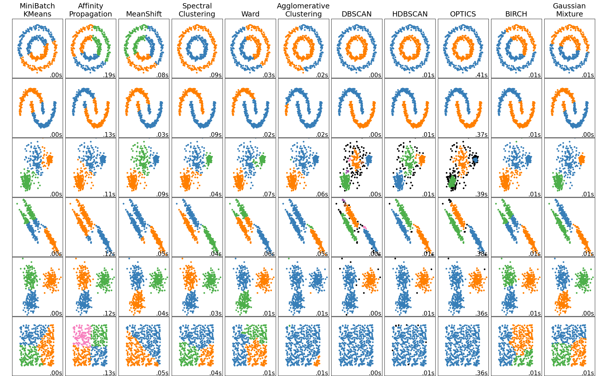
Hinh: So sanh cac thuat toan clustering tren cac loai data khac nhau.
📝 Tổng Kết
Key Takeaways:
- 📊 Unsupervised Learning học patterns từ data không có label
- 🎯 K-Means là clustering algorithm đơn giản nhất, dùng Elbow để chọn k
- 📉 PCA giảm chiều giữ maximum variance
- 🔍 Anomaly Detection (Isolation Forest) phát hiện fraud/outlier
- 💻 Scikit-learn:
KMeans(),PCA(),IsolationForest()
Bài tập tự luyện
- Bài tập 1: Implement K-Means từ đầu (không dùng sklearn)
- Bài tập 2: Áp dụng PCA để giảm MNIST từ 784D xuống 2D, visualize
- Bài tập 3: Sử dụng Isolation Forest phát hiện fraud trong credit card data
Tài liệu tham khảo
| Nguồn | Link |
|---|---|
| Scikit-learn Clustering | scikit-learn.org |
| Scikit-learn PCA | scikit-learn.org |
| Understanding K-Means | towardsdatascience.com |
Câu hỏi tự kiểm tra
- Unsupervised Learning khác Supervised Learning ở điểm nào? Cho ví dụ bài toán phù hợp với mỗi loại.
- Thuật toán K-Means chọn số cluster k như thế nào? Elbow Method hoạt động ra sao?
- PCA giảm chiều dữ liệu bằng cách nào mà vẫn giữ được maximum variance?
- Isolation Forest phát hiện anomaly (bất thường) dựa trên nguyên lý gì?
🎉 Tuyệt vời! Bạn đã hoàn thành bài học Unsupervised Learning!
Tiếp theo: Cùng học Ensemble Methods — kết hợp nhiều models để đạt hiệu suất cao nhất!
Checkpoint
Bạn đã nắm vững Unsupervised Learning chưa? Sẵn sàng sang Ensemble Methods!