🎯 Mục tiêu bài học
Sau bài học này, học viên sẽ:
✅ Hiểu Sigmoid Function và cách chuyển đổi z-score thành probability
✅ Nắm vững Log-Odds (Logit) và Decision Boundary
✅ Tính toán thủ công probabilities và thresholds
✅ Implement với Scikit-learn đầy đủ workflow
✅ Hiểu Confusion Matrix, Precision, Recall, F1-Score
✅ Vẽ và phân tích ROC Curve & AUC
✅ Áp dụng Regularization (L1/L2)
Thời gian: 4-5 giờ | Độ khó: Theory
� Bảng Thuật Ngữ Quan Trọng
| Thuật ngữ | Tiếng Việt | Giải thích đơn giản |
|---|---|---|
| Logistic Regression | Hồi quy logistic | Thuật toán classification dùng sigmoid |
| Sigmoid Function | Hàm sigmoid | Chuyển số thực thành probability [0,1] |
| Log-Odds (Logit) | Log tỷ số | — đại lượng tuyến tính |
| Decision Boundary | Biên quyết định | Ngưỡng phân chia 2 class (mặc định p=0.5) |
| Confusion Matrix | Ma trận nhầm lẫn | Bảng TP/FP/TN/FN đánh giá classification |
| Precision | Độ chính xác | Tỷ lệ dự đoán dương đúng trong số dự đoán dương |
| Recall | Độ phủ | Tỷ lệ tìm được trong số thực tế dương |
| ROC Curve | Đường ROC | Biểu đồ TPR vs FPR ở các threshold khác nhau |
Checkpoint
Bạn đã đọc qua bảng thuật ngữ? Hãy ghi nhớ chúng!
�📐 The Model - Lý thuyết cốt lõi
Lưu ý: Mặc dù có từ "Regression" trong tên, nhưng Logistic Regression được dùng cho Classification (Phân loại), KHÔNG phải Regression!
1.1 The Sigmoid Function
Sigmoid Function chuyển đổi bất kỳ giá trị thực z nào thành probability trong khoảng [0, 1]:
Đặc điểm:
- Input z: Bất kỳ số thực nào ( đến )
- Output p: Luôn trong [0, 1] - có thể diễn giải như xác suất
- Threshold mặc định: 0.5
- Nếu → Dự đoán Class 1 (Positive/Yes/True)
- Nếu → Dự đoán Class 0 (Negative/No/False)
1import numpy as np2import matplotlib.pyplot as plt34# Sigmoid function5def sigmoid(z):6 return 1 / (1 + np.exp(-z))78# Plot9z = np.linspace(-10, 10, 100)10p = sigmoid(z)1112plt.figure(figsize=(10, 6))13plt.plot(z, p, 'b-', linewidth=2)14plt.axhline(0.5, color='r', linestyle='--', label='Threshold = 0.5')15plt.axvline(0, color='gray', linestyle='--', alpha=0.5)16plt.xlabel('z (Linear Combination)', fontsize=12)17plt.ylabel('p (Probability)', fontsize=12)18plt.title('Sigmoid Function', fontsize=14)19plt.grid(alpha=0.3)20plt.legend()21plt.show()1.2 The Linear Part - Decision Boundary
Phần tuyến tính bên trong sigmoid định nghĩa Decision Boundary:
Trong đó:
- : Intercept (bias term)
- : Coefficients (weights)
- : Features
Decision Boundary là đường thẳng/mặt phẳng tại (tương ứng ).
1.3 Log-Odds (Logit)
Model thực tế dự đoán log-odds (logarit của tỷ lệ cược) của lớp positive:
Giải thích:
- : Odds - tỷ lệ giữa xác suất xảy ra và không xảy ra
- Nếu odds = 2 → Khả năng xảy ra gấp 2 lần không xảy ra
- : Log-odds có thể nhận giá trị từ đến
Checkpoint
Bạn đã hiểu cách Sigmoid chuyển đổi z-score thành probability chưa?
📝 Ví dụ tính toán thủ công
3. Ví dụ tính toán thủ công
3.1 Bai toan
Du doan benh nhan co bi benh tim khong dua tren tuoi.
Du lieu:
| Tuoi (x) | Benh tim (y) |
|---|---|
| 30 | 0 |
| 35 | 0 |
| 40 | 0 |
| 45 | 1 |
| 50 | 1 |
| 55 | 1 |
| 60 | 1 |
Gia su sau khi train, ta co: ,
3.2 Tinh xac suat cho tuoi 50
Buoc 1: Tinh z
Buoc 2: Ap dung Sigmoid
3.3 Tinh xac suat cho tuoi 60
Buoc 1: Tinh z
Buoc 2: Ap dung Sigmoid
3.4 Tinh xac suat cho tuoi 40
3.5 Decision Boundary
Voi threshold = 0.5:
| Tuoi | P(y=1) | Du doan |
|---|---|---|
| 30 | 0.12 | 0 (Khong benh) |
| 40 | 0.27 | 0 (Khong benh) |
| 50 | 0.50 | Giap ranh |
| 60 | 0.73 | 1 (Co benh) |
| 70 | 0.88 | 1 (Co benh) |
📉 Loss Function: Cross-Entropy
4. Loss Function: Cross-Entropy
4.1 Binary Cross-Entropy Loss
4.2 Y nghia
- Khi : Loss = (muon gan 1)
- Khi : Loss = (muon gan 0)
💻 Scikit-Learn Workflow
2. Scikit-Learn Workflow - Thực hành đầy đủ
Quy trình Logistic Regression với Scikit-Learn
2.1 Setup & Scaling
Quan trọng: Logistic Regression yêu cầu scaling để đảm bảo convergence (hội tụ)!
1from sklearn.linear_model import LogisticRegression2from sklearn.preprocessing import StandardScaler3from sklearn.model_selection import train_test_split45# Split data6X_train, X_test, y_train, y_test = train_test_split(7 X, y, test_size=0.2, random_state=428)910# Scale features (CRITICAL!)11scaler = StandardScaler()12# Fit on TRAIN, transform BOTH13X_train_scaled = scaler.fit_transform(X_train)14X_test_scaled = scaler.transform(X_test)2.2 Train Model
1# Instantiate model2model = LogisticRegression()34# Fit (train)5model.fit(X_train_scaled, y_train)67# Check coefficients8print(f"Coefficients: {model.coef_}")9print(f"Intercept: {model.intercept_}")2.3 Predictions
Logistic Regression cho 2 loại output:
1# Get Class labels (0 or 1)2y_pred = model.predict(X_test_scaled)3print(f"Predicted Classes: {y_pred[:5]}")4# Output: [0 1 1 0 1]56# Get Probabilities [P(Class 0), P(Class 1)]7y_prob = model.predict_proba(X_test_scaled)8print(f"Probabilities:\n{y_prob[:5]}")9# Output:10# [[0.89 0.11] # 89% Class 0, 11% Class 111# [0.23 0.77] # 23% Class 0, 77% Class 112# ...]1314# Get only P(Class 1) - for ROC curve15y_prob_pos = y_prob[:, 1]Checkpoint
Bạn đã hiểu workflow train và predict với Scikit-learn chưa?
📊 Confusion Matrix
3. Confusion Matrix - Nền tảng của Classification Metrics
Confusion Matrix là bảng mô tả hiệu suất của classifier:
1PREDICTED CLASS2 0 (Neg) 1 (Pos)3ACTUAL 0 (Neg) TN FP4CLASS 1 (Pos) FN TP4 thành phần:
- TN (True Negative): Dự đoán 0, thực tế 0 ✅ (Correct)
- FP (False Positive): Dự đoán 1, thực tế 0 ❌ (Type I Error - False Alarm)
- FN (False Negative): Dự đoán 0, thực tế 1 ❌ (Type II Error - Miss)
- TP (True Positive): Dự đoán 1, thực tế 1 ✅ (Correct)
1from sklearn.metrics import confusion_matrix, classification_report23# Generate confusion matrix4cm = confusion_matrix(y_test, y_pred)5print(cm)6# Output:7# [[50 5] <- 50 TN, 5 FP8# [ 3 42]] <- 3 FN, 42 TP910# Visualize11import seaborn as sns12import matplotlib.pyplot as plt1314plt.figure(figsize=(8, 6))15sns.heatmap(cm, annot=True, fmt='d', cmap='Blues', 16 xticklabels=['Negative', 'Positive'],17 yticklabels=['Negative', 'Positive'])18plt.xlabel('Predicted')19plt.ylabel('Actual')20plt.title('Confusion Matrix')21plt.show()3.1 Metrics từ Confusion Matrix
1. Precision (Độ chính xác - Quality)
"Trong tất cả dự đoán Positive, bao nhiêu % là đúng?"
Mục tiêu: Minimize False Alarms (FP)
2. Recall / Sensitivity (Độ bao phủ - Quantity)
"Trong tất cả Positive thực tế, bao nhiêu % được tìm thấy?"
Mục tiêu: Minimize Misses (FN)
3. F1-Score (Harmonic Mean)
Best balance cho imbalanced data
4. Accuracy
Cảnh báo: Tốt cho balanced datasets. Không tốt cho imbalanced data!
1from sklearn.metrics import classification_report23print(classification_report(y_test, y_pred))4# Output:5# precision recall f1-score support6#7# 0 0.94 0.91 0.93 558# 1 0.89 0.93 0.91 459#10# accuracy 0.92 10011# macro avg 0.92 0.92 0.92 10012# weighted avg 0.92 0.92 0.92 100📈 ROC & Thresholds
4. ROC & Thresholds - Đánh giá model across ALL thresholds
4.1 Vấn đề với Threshold cố định
Mặc định threshold = 0.5, nhưng:
- Medical diagnosis: Muốn Recall cao → Threshold thấp (0.3)
- Spam filter: Muốn Precision cao → Threshold cao (0.7)
ROC Curve đánh giá model performance ở TẤT CẢ thresholds!
4.2 ROC Curve (Receiver Operating Characteristic)
ROC Curve vẽ:
- TPR (True Positive Rate) = Recall trên trục Y
- FPR (False Positive Rate) = False Alarm Rate trên trục X
1from sklearn.metrics import roc_curve, roc_auc_score2import matplotlib.pyplot as plt34# Get probabilities for positive class5y_prob = model.predict_proba(X_test_scaled)[:, 1]67# Calculate ROC curve8fpr, tpr, thresholds = roc_curve(y_test, y_prob)910# Calculate AUC11auc = roc_auc_score(y_test, y_prob)1213# Plot ROC Curve14plt.figure(figsize=(10, 8))15plt.plot(fpr, tpr, 'b-', linewidth=2, label=f'Model (AUC = {auc:.2f})')16plt.plot([0, 1], [0, 1], 'r--', label='Random Guess (AUC = 0.5)')17plt.xlabel('False Positive Rate (FPR)', fontsize=12)18plt.ylabel('True Positive Rate (TPR / Recall)', fontsize=12)19plt.title('ROC Curve', fontsize=14)20plt.legend()21plt.grid(alpha=0.3)22plt.show()2324print(f"AUC Score: {auc:.4f}")4.3 AUC (Area Under Curve)
AUC = Diện tích dưới ROC Curve
Giải thích:
- AUC = 0.5: Random guessing (đường chéo)
- AUC = 1.0: Perfect classifier
- AUC > 0.8: Generally considered good
- AUC > 0.9: Excellent
Ý nghĩa: Xác suất model rank một sample Positive ngẫu nhiên cao hơn một sample Negative ngẫu nhiên
1# Use probabilities, NOT class labels!2auc_score = roc_auc_score(y_test, y_prob)3print(f"AUC: {auc_score:.4f}")Checkpoint
Bạn có thể giải thích ý nghĩa của AUC = 0.85 không?
🎯 Multiclass Strategy
5. Multiclass Strategy
5.1 One-vs-Rest (OvR) - Mặc định trong Scikit-Learn
Train K classifiers nhị phân, mỗi model phân biệt 1 class với tất cả class khác.
1# Default strategy2model = LogisticRegression() # multi_class='auto' -> OvR3model.fit(X, y)Ưu điểm:
- Interpretable (dễ giải thích)
- Nhanh
5.2 Multinomial (Softmax) - Tốt hơn cho multiclass
Softmax generalizes sigmoid cho nhiều classes, probabilities tổng = 1:
1from sklearn.datasets import load_iris23# Load data4iris = load_iris()5X, y = iris.data, iris.target67# Train multiclass với Softmax8model = LogisticRegression(9 multi_class='multinomial', # Use Softmax10 solver='lbfgs', # Required for multinomial11 max_iter=100012)13model.fit(X, y)1415# Predict probabilities for all classes16probs = model.predict_proba(X[:5])17print(f"Probabilities (sum to 1.0):\n{probs}")18# Output:19# [[0.90 0.08 0.02] <- 90% Class 0, 8% Class 1, 2% Class 220# [0.75 0.20 0.05]21# ...]⚠️ Key Assumptions
6. Key Assumptions - Giả định quan trọng
Để Logistic Regression hoạt động tốt, cần đảm bảo:
| # | Assumption | Mô tả | Hậu quả nếu vi phạm |
|---|---|---|---|
| 1 | Binary Outcome | Target là 0 hoặc 1 | Model không train được |
| 2 | Independence | Observations độc lập | Confidence intervals sai |
| 3 | Little Multicollinearity | Features không highly correlated | Coefficients không ổn định |
| 4 | Linearity of Log-Odds | Quan hệ tuyến tính giữa X và log-odds | Poor fit |
| 5 | Large Sample Size | Đủ lớn để stable | Coefficients không reliable |
6.1 Kiểm tra Multicollinearity
1import pandas as pd2import numpy as np34# Calculate correlation matrix5df = pd.DataFrame(X, columns=['Feature1', 'Feature2', 'Feature3'])6corr = df.corr()78# Visualize9import seaborn as sns10sns.heatmap(corr, annot=True, cmap='coolwarm', center=0)11plt.title('Feature Correlation Matrix')12plt.show()1314# Rule: Correlation > 0.8 → Multicollinearity problem!🔧 Regularization - L1 & L2
7. Regularization - L1 & L2
7.1 Lý thuyết
| Type | Formula | Effect | Use case |
|---|---|---|---|
| L2 (Ridge) | Giảm overfitting | Mặc định, tốt nhất | |
| L1 (Lasso) | Feature selection (force some β=0) | Nhiều features không quan trọng | |
| Elastic Net | Kết hợp L1 & L2 | Multicollinearity |
7.2 Code với Scikit-Learn
1# L2 Regularization (default, best)2model_l2 = LogisticRegression(3 penalty='l2', # Ridge4 C=1.0, # C = 1/λ (C nhỏ = regularization mạnh)5 solver='lbfgs'6)78# L1 Regularization (feature selection)9model_l1 = LogisticRegression(10 penalty='l1', # Lasso11 C=0.5, # Stronger regularization12 solver='saga' # Required for L113)1415# Elastic Net16model_en = LogisticRegression(17 penalty='elasticnet',18 l1_ratio=0.5, # 0.5 = 50% L1, 50% L219 solver='saga',20 C=1.021)2223# Compare24for model, name in [(model_l2, 'L2'), (model_l1, 'L1')]:25 model.fit(X_train_scaled, y_train)26 score = model.score(X_test_scaled, y_test)27 print(f"{name} Accuracy: {score:.4f}")Parameter C:
- C lớn (e.g., 10): Regularization yếu → Risk of overfitting
- C nhỏ (e.g., 0.1): Regularization mạnh → Risk of underfitting
- C = 1.0: Mặc định, thường tốt
⚖️ Ưu và Nhược điểm
8. Ưu và Nhược điểm
| ✅ Ưu điểm | ❌ Nhược điểm |
|---|---|
| Đơn giản, nhanh | Chỉ tốt cho linearly separable data |
| Output = probabilities (0-1) | Không capture non-linear relationships |
| Dễ interpret (odds ratio) | Cần feature engineering cho complex patterns |
| Ít bị overfitting | Giả định independence của features |
| Regularization built-in (L1/L2) | Yêu cầu scaling |
| Multiclass support | Kém hơn tree-based với outliers |
8.1 Khi nào dùng Logistic Regression?
✅ Sử dụng khi:
- Data linearly separable hoặc gần linearly separable
- Cần probabilities chính xác (medical, credit scoring)
- Cần model interpretable (banking, legal)
- Dataset nhỏ đến trung bình
❌ KHÔNG sử dụng khi:
- Relationships rất non-linear (dùng Decision Tree, Neural Networks)
- Features highly correlated (dùng PCA trước hoặc Ridge Regression)
- Outliers nhiều (dùng Tree-based models) |---------|------------| | Don gian, nhanh | Chi tot cho linearly separable | | Output la xac suat | Khong capture non-linear relationships | | De interpret (odds ratio) | Can feature engineering | | It bi overfitting | Gia dinh independence cua features |
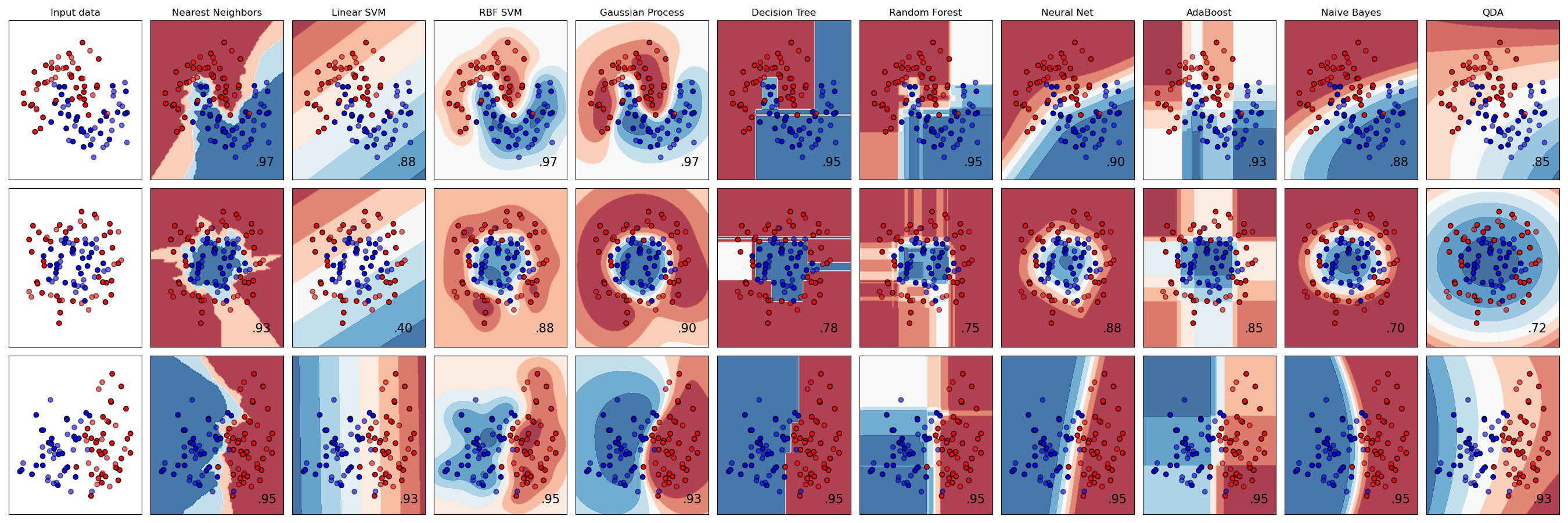
Hinh: So sanh decision boundary cua cac classifier
📝 Tổng Kết
Key Takeaways:
- 📊 Logistic Regression dùng Sigmoid chuyển z-score → probability
- 🎯 Decision Boundary mặc định tại p = 0.5, có thể điều chỉnh threshold
- 📏 Đánh giá: Confusion Matrix, Precision, Recall, F1-Score, ROC-AUC
- ⚖️ Regularization: L1 (sparse features), L2 (s hrink coefficients)
- 💻 Scikit-learn:
LogisticRegression(C=1.0, penalty='l2')
Bài tập tự luyện
- Bài 1: Tính thủ công P(y=1) khi β₀=-3, β₁=0.5, x=8
- Bài 2: Train Logistic Regression trên Titanic dataset, đánh giá accuracy
- Bài 3: So sánh L1 và L2 regularization trên cùng dataset
Tài liệu tham khảo
| Nguồn | Link |
|---|---|
| Scikit-learn Logistic Regression | scikit-learn.org |
| StatQuest - Logistic Regression | youtube.com |
Câu hỏi tự kiểm tra
- Sigmoid Function chuyển đổi z-score thành probability như thế nào? Tại sao cần hàm này?
- Decision Boundary mặc định là p = 0.5 — khi nào cần điều chỉnh threshold khác?
- Phân biệt Precision và Recall — trong bài toán phát hiện bệnh, metric nào quan trọng hơn?
- L1 và L2 Regularization khác nhau như thế nào? Khi nào dùng L1?
🎉 Tuyệt vời! Bạn đã hoàn thành bài học Logistic Regression!
Tiếp theo: Cùng học Decision Tree — thuật toán trực quan và mạnh mẽ!
Checkpoint
Bạn đã nắm vững Logistic Regression chưa? Sẵn sàng sang Decision Tree!